對其中的參數(shù)進行解釋

plt.subplots(figsize=(9, 9))設(shè)置畫面大小，會使得整個畫面等比例放大的

sns.heapmap()這個當然是用來生成熱力圖的啦

df是DataFrame， pandas的這個類還是很常用的啦~

df.corr()就是得到這個dataframe的相關(guān)系數(shù)矩陣

把這個矩陣直接丟給sns.heapmap中做參數(shù)就好啦

sns.heapmap中annot=True，意思是顯式熱力圖上的數(shù)值大小。

sns.heapmap中square=True，意思是將圖變成一個正方形，默認是一個矩形

sns.heapmap中cmap='Blues'是一種模式，就是圖顏色配置方案啦，我很喜歡這一款的。

sns.heapmap中vmax是顯示最大值

import seaborn as snsimport matplotlib.pyplot as pltdef test(df): dfData = df.corr() plt.subplots(figsize=(9, 9)) # 設(shè)置畫面大小 sns.heatmap(dfData, annot=True, vmax=1, square=True, cmap='Blues') plt.savefig(’./BluesStateRelation.png’) plt.show()

補充知識：python混淆矩陣（confusion_matrix）FP、FN、TP、TN、ROC，精確率(Precision),召回率(Recall),準確率(Accuracy)詳述與實現(xiàn)

一、FP、FN、TP、TN

你這蠢貨，是不是又把酸葡萄和葡萄酸弄“混淆“”啦！！！

上面日常情況中的混淆就是：是否把某兩件東西或者多件東西給弄混了，迷糊了。

在機器學(xué)習(xí)中, 混淆矩陣是一個誤差矩陣, 常用來可視化地評估監(jiān)督學(xué)習(xí)算法的性能.。混淆矩陣大小為 (n_classes, n_classes) 的方陣, 其中 n_classes 表示類的數(shù)量。

其中，這個矩陣的一行表示預(yù)測類中的實例（可以理解為模型預(yù)測輸出，predict），另一列表示對該預(yù)測結(jié)果與標簽（Ground Truth）進行判定模型的預(yù)測結(jié)果是否正確，正確為True，反之為False。

在機器學(xué)習(xí)中g(shù)round truth表示有監(jiān)督學(xué)習(xí)的訓(xùn)練集的分類準確性，用于證明或者推翻某個假設(shè)。有監(jiān)督的機器學(xué)習(xí)會對訓(xùn)練數(shù)據(jù)打標記，試想一下如果訓(xùn)練標記錯誤，那么將會對測試數(shù)據(jù)的預(yù)測產(chǎn)生影響，因此這里將那些正確打標記的數(shù)據(jù)成為ground truth。

此時，就引入FP、FN、TP、TN與精確率(Precision)，召回率(Recall)，準確率(Accuracy)。

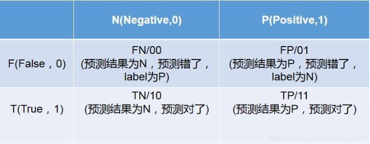
以貓狗二分類為例，假定cat為正例-Positive，dog為負例-Negative；預(yù)測正確為True，反之為False。我們就可以得到下面這樣一個表示FP、FN、TP、TN的表：

此時如下代碼所示，其中scikit-learn 混淆矩陣函數(shù) sklearn.metrics.confusion_matrix API 接口，可以用于繪制混淆矩陣

skearn.metrics.confusion_matrix( y_true, # array, Gound true (correct) target values y_pred, # array, Estimated targets as returned by a classifier labels=None, # array, List of labels to index the matrix. sample_weight=None # array-like of shape = [n_samples], Optional sample weights)

完整示例代碼如下：

__author__ = 'lingjun'# welcome to attention:小白CV import seaborn as snsfrom sklearn.metrics import confusion_matriximport matplotlib.pyplot as pltsns.set() f, (ax1,ax2) = plt.subplots(figsize = (10, 8),nrows=2)y_true = ['dog', 'dog', 'dog', 'cat', 'cat', 'cat', 'cat']y_pred = ['cat', 'cat', 'dog', 'cat', 'cat', 'cat', 'cat']C2= confusion_matrix(y_true, y_pred, labels=['dog', 'cat'])print(C2)print(C2.ravel())sns.heatmap(C2,annot=True) ax2.set_title(’sns_heatmap_confusion_matrix’)ax2.set_xlabel(’Pred’)ax2.set_ylabel(’True’)f.savefig(’sns_heatmap_confusion_matrix.jpg’, bbox_inches=’tight’)

保存的圖像如下所示：

這個時候我們還是不知道skearn.metrics.confusion_matrix做了些什么，這個時候print(C2)，打印看下C2究竟里面包含著什么。最終的打印結(jié)果如下所示：

[[1 2] [0 4]][1 2 0 4]

解釋下上面這幾個數(shù)字的意思：

C2= confusion_matrix(y_true, y_pred, labels=['dog', 'cat'])中的labels的順序就分布是0、1，negative和positive

注：labels=[]可加可不加，不加情況下會自動識別，自己定義

cat為1-positive，其中真實值中cat有4個，4個被預(yù)測為cat，預(yù)測正確T，0個被預(yù)測為dog，預(yù)測錯誤F；

dog為0-negative，其中真實值中dog有3個，1個被預(yù)測為dog，預(yù)測正確T，2個被預(yù)測為cat，預(yù)測錯誤F。

所以：TN=1、 FP=2 、FN=0、TP=4。

TN=1：預(yù)測為negative狗中1個被預(yù)測正確了

FP=2 ：預(yù)測為positive貓中2個被預(yù)測錯誤了

FN=0：預(yù)測為negative狗中0個被預(yù)測錯誤了

TP=4：預(yù)測為positive貓中4個被預(yù)測正確了

這時候再把上面貓狗預(yù)測結(jié)果拿來看看，6個被預(yù)測為cat，但是只有4個的true是cat，此時就和右側(cè)的紅圈對應(yīng)上了。

y_pred = ['cat', 'cat', 'dog', 'cat', 'cat', 'cat', 'cat']y_true = ['dog', 'dog', 'dog', 'cat', 'cat', 'cat', 'cat']

二、精確率(Precision),召回率(Recall),準確率(Accuracy)

有了上面的這些數(shù)值，就可以進行如下的計算工作了

準確率(Accuracy):這三個指標里最直觀的就是準確率: 模型判斷正確的數(shù)據(jù)(TP+TN)占總數(shù)據(jù)的比例

'Accuracy: '+str(round((tp+tn)/(tp+fp+fn+tn), 3))

召回率(Recall): 針對數(shù)據(jù)集中的所有正例label(TP+FN)而言,模型正確判斷出的正例(TP)占數(shù)據(jù)集中所有正例的比例；FN表示被模型誤認為是負例但實際是正例的數(shù)據(jù)；召回率也叫查全率，以物體檢測為例,我們往往把圖片中的物體作為正例，此時召回率高代表著模型可以找出圖片中更多的物體!

'Recall: '+str(round((tp)/(tp+fn), 3))

精確率(Precision):針對模型判斷出的所有正例(TP+FP)而言，其中真正例(TP)占的比例。精確率也叫查準率,還是以物體檢測為例，精確率高表示模型檢測出的物體中大部分確實是物體，只有少量不是物體的對象被當成物體。

'Precision: '+str(round((tp)/(tp+fp), 3))

還有：

('Sensitivity: '+str(round(tp/(tp+fn+0.01), 3)))('Specificity: '+str(round(1-(fp/(fp+tn+0.01)), 3)))('False positive rate: '+str(round(fp/(fp+tn+0.01), 3)))('Positive predictive value: '+str(round(tp/(tp+fp+0.01), 3)))('Negative predictive value: '+str(round(tn/(fn+tn+0.01), 3)))

三.繪制ROC曲線，及計算以上評價參數(shù)

如下為統(tǒng)計數(shù)據(jù)：

__author__ = 'lingjun'# E-mail: 1763469890@qq.com from sklearn.metrics import roc_auc_score, confusion_matrix, roc_curve, aucfrom matplotlib import pyplot as pltimport numpy as npimport torchimport csv def confusion_matrix_roc(GT, PD, experiment, n_class): GT = GT.numpy() PD = PD.numpy() y_gt = np.argmax(GT, 1) y_gt = np.reshape(y_gt, [-1]) y_pd = np.argmax(PD, 1) y_pd = np.reshape(y_pd, [-1]) # ---- Confusion Matrix and Other Statistic Information ---- if n_class > 2: c_matrix = confusion_matrix(y_gt, y_pd) # print('Confussion Matrix:n', c_matrix) list_cfs_mtrx = c_matrix.tolist() # print('List', type(list_cfs_mtrx[0])) path_confusion = r'./records/' + experiment + '/confusion_matrix.txt' # np.savetxt(path_confusion, (c_matrix)) np.savetxt(path_confusion, np.reshape(list_cfs_mtrx, -1), delimiter=’,’, fmt=’%5s’) if n_class == 2: list_cfs_mtrx = [] tn, fp, fn, tp = confusion_matrix(y_gt, y_pd).ravel() list_cfs_mtrx.append('TN: ' + str(tn)) list_cfs_mtrx.append('FP: ' + str(fp)) list_cfs_mtrx.append('FN: ' + str(fn)) list_cfs_mtrx.append('TP: ' + str(tp)) list_cfs_mtrx.append(' ') list_cfs_mtrx.append('Accuracy: ' + str(round((tp + tn) / (tp + fp + fn + tn), 3))) list_cfs_mtrx.append('Sensitivity: ' + str(round(tp / (tp + fn + 0.01), 3))) list_cfs_mtrx.append('Specificity: ' + str(round(1 - (fp / (fp + tn + 0.01)), 3))) list_cfs_mtrx.append('False positive rate: ' + str(round(fp / (fp + tn + 0.01), 3))) list_cfs_mtrx.append('Positive predictive value: ' + str(round(tp / (tp + fp + 0.01), 3))) list_cfs_mtrx.append('Negative predictive value: ' + str(round(tn / (fn + tn + 0.01), 3))) path_confusion = r'./records/' + experiment + '/confusion_matrix.txt' np.savetxt(path_confusion, np.reshape(list_cfs_mtrx, -1), delimiter=’,’, fmt=’%5s’) # ---- ROC ---- plt.figure(1) plt.figure(figsize=(6, 6)) fpr, tpr, thresholds = roc_curve(GT[:, 1], PD[:, 1]) roc_auc = auc(fpr, tpr) plt.plot(fpr, tpr, lw=1, label='ATB vs NotTB, area=%0.3f)' % (roc_auc)) # plt.plot(thresholds, tpr, lw=1, label=’Thr%d area=%0.2f)’ % (1, roc_auc)) # plt.plot([0, 1], [0, 1], ’--’, color=(0.6, 0.6, 0.6), label=’Luck’) plt.xlim([0.00, 1.0]) plt.ylim([0.00, 1.0]) plt.xlabel('False Positive Rate') plt.ylabel('True Positive Rate') plt.title('ROC') plt.legend(loc='lower right') plt.savefig(r'./records/' + experiment + '/ROC.png') print('ok') def inference(): GT = torch.FloatTensor() PD = torch.FloatTensor() file = r'Sensitive_rename_inform.csv' with open(file, ’r’, encoding=’UTF-8’) as f: reader = csv.DictReader(f) for row in reader: # TODO max_patient_score = float(row[’ai1’]) doctor_gt = row[’gt2’] print(max_patient_score,doctor_gt) pd = [[max_patient_score, 1-max_patient_score]] output_pd = torch.FloatTensor(pd).to(device) if doctor_gt == '+': target = [[1.0, 0.0]] else: target = [[0.0, 1.0]] target = torch.FloatTensor(target) # 類型轉(zhuǎn)換, 將list轉(zhuǎn)化為tensor, torch.FloatTensor([1,2]) Target = torch.autograd.Variable(target).long().to(device) GT = torch.cat((GT, Target.float().cpu()), 0) # 在行上進行堆疊 PD = torch.cat((PD, output_pd.float().cpu()), 0) confusion_matrix_roc(GT, PD, 'ROC', 2) if __name__ == '__main__': inference()

若是表格里面有中文，則記得這里進行修改，否則報錯

with open(file, ’r’) as f:

以上這篇Python數(shù)據(jù)相關(guān)系數(shù)矩陣和熱力圖輕松實現(xiàn)教程就是小編分享給大家的全部內(nèi)容了，希望能給大家一個參考，也希望大家多多支持好吧啦網(wǎng)。