python實現梯度下降算法的實例詳解
python版本選擇
這里選的python版本是2.7,因為我之前用python3試了幾次,發現在畫3d圖的時候會報錯,所以改用了2.7。
數據集選擇
數據集我選了一個包含兩個變量,三個參數的數據集,這樣可以畫出3d圖形對結果進行驗證。
部分函數總結
symbols()函數:首先要安裝sympy庫才可以使用。用法:
>>> x1 = symbols(’x2’)>>> x1 + 1x2 + 1
在這個例子中,x1和x2是不一樣的,x2代表的是一個函數的變量,而x1代表的是python中的一個變量,它可以表示函數的變量,也可以表示其他的任何量,它替代x2進行函數的計算。實際使用的時候我們可以將x1,x2都命名為x,但是我們要知道他們倆的區別。再看看這個例子:
>>> x = symbols(’x’)>>> expr = x + 1>>> x = 2>>> print(expr)x + 1
作為python變量的x被2這個數值覆蓋了,所以它現在不再表示函數變量x,而expr依然是函數變量x+1的別名,所以結果依然是x+1。subs()函數:既然普通的方法無法為函數變量賦值,那就肯定有函數來實現這個功能,用法:
>>> (1 + x*y).subs(x, pi)#一個參數時的用法pi*y + 1>>> (1 + x*y).subs({x:pi, y:2})#多個參數時的用法1 + 2*pi
diff()函數:求偏導數,用法:result=diff(fun,x),這個就是求fun函數對x變量的偏導數,結果result也是一個變量,需要賦值才能得到準確結果。
代碼實現:
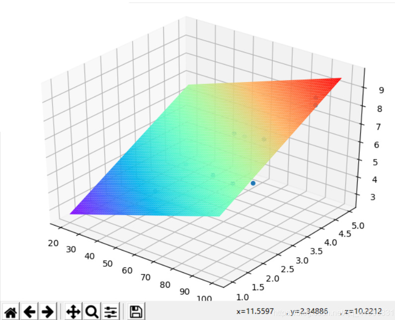
from __future__ import divisionfrom sympy import symbols, diff, expandimport numpy as npimport matplotlib.pyplot as pltfrom mpl_toolkits.mplot3d import Axes3Ddata = {’x1’: [100, 50, 100, 100, 50, 80, 75, 65, 90, 90],’x2’: [4, 3, 4, 2, 2, 2, 3, 4, 3, 2],’y’: [9.3, 4.8, 8.9, 6.5, 4.2, 6.2, 7.4, 6.0, 7.6, 6.1]}#初始化數據集theta0, theta1, theta2 = symbols(’theta0 theta1 theta2’, real=True) # y=theta0+theta1*x1+theta2*x2,定義參數costfuc = 0 * theta0for i in range(10): costfuc += (theta0 + theta1 * data[’x1’][i] + theta2 * data[’x2’][i] - data[’y’][i]) ** 2costfuc /= 20#初始化代價函數dtheta0 = diff(costfuc, theta0)dtheta1 = diff(costfuc, theta1)dtheta2 = diff(costfuc, theta2)rtheta0 = 1rtheta1 = 1rtheta2 = 1#為參數賦初始值costvalue = costfuc.subs({theta0: rtheta0, theta1: rtheta1, theta2: rtheta2})newcostvalue = 0#用cost的值的變化程度來判斷是否已經到最小值了count = 0alpha = 0.0001#設置學習率,一定要設置的比較小,否則無法到達最小值while (costvalue - newcostvalue > 0.00001 or newcostvalue - costvalue > 0.00001) and count < 1000: count += 1 costvalue = newcostvalue rtheta0 = rtheta0 - alpha * dtheta0.subs({theta0: rtheta0, theta1: rtheta1, theta2: rtheta2}) rtheta1 = rtheta1 - alpha * dtheta1.subs({theta0: rtheta0, theta1: rtheta1, theta2: rtheta2}) rtheta2 = rtheta2 - alpha * dtheta2.subs({theta0: rtheta0, theta1: rtheta1, theta2: rtheta2}) newcostvalue = costfuc.subs({theta0: rtheta0, theta1: rtheta1, theta2: rtheta2})rtheta0 = round(rtheta0, 4)rtheta1 = round(rtheta1, 4)rtheta2 = round(rtheta2, 4)#給結果保留4位小數,防止數值溢出print(rtheta0, rtheta1, rtheta2)fig = plt.figure()ax = Axes3D(fig)ax.scatter(data[’x1’], data[’x2’], data[’y’]) # 繪制散點圖xx = np.arange(20, 100, 1)yy = np.arange(1, 5, 0.05)X, Y = np.meshgrid(xx, yy)Z = X * rtheta1 + Y * rtheta2 + rtheta0ax.plot_surface(X, Y, Z, rstride=1, cstride=1, cmap=plt.get_cmap(’rainbow’))plt.show()#繪制3d圖進行驗證
結果:

實例擴展:
’’’梯度下降算法Batch Gradient DescentStochastic Gradient Descent SGD’’’__author__ = ’epleone’import numpy as npimport matplotlib.pyplot as pltfrom mpl_toolkits.mplot3d import Axes3Dimport sys# 使用隨機數種子, 讓每次的隨機數生成相同,方便調試# np.random.seed(111111111)class GradientDescent(object): eps = 1.0e-8 max_iter = 1000000 # 暫時不需要 dim = 1 func_args = [2.1, 2.7] # [w_0, .., w_dim, b] def __init__(self, func_arg=None, N=1000): self.data_num = N if func_arg is not None: self.FuncArgs = func_arg self._getData() def _getData(self): x = 20 * (np.random.rand(self.data_num, self.dim) - 0.5) b_1 = np.ones((self.data_num, 1), dtype=np.float) # x = np.concatenate((x, b_1), axis=1) self.x = np.concatenate((x, b_1), axis=1) def func(self, x): # noise太大的話, 梯度下降法失去作用 noise = 0.01 * np.random.randn(self.data_num) + 0 w = np.array(self.func_args) # y1 = w * self.x[0, ] # 直接相乘 y = np.dot(self.x, w) # 矩陣乘法 y += noise return y @property def FuncArgs(self): return self.func_args @FuncArgs.setter def FuncArgs(self, args): if not isinstance(args, list): raise Exception( ’args is not list, it should be like [w_0, ..., w_dim, b]’) if len(args) == 0: raise Exception(’args is empty list!!’) if len(args) == 1: args.append(0.0) self.func_args = args self.dim = len(args) - 1 self._getData() @property def EPS(self): return self.eps @EPS.setter def EPS(self, value): if not isinstance(value, float) and not isinstance(value, int): raise Exception('The type of eps should be an float number') self.eps = value def plotFunc(self): # 一維畫圖 if self.dim == 1: # x = np.sort(self.x, axis=0) x = self.x y = self.func(x) fig, ax = plt.subplots() ax.plot(x, y, ’o’) ax.set(xlabel=’x ’, ylabel=’y’, title=’Loss Curve’) ax.grid() plt.show() # 二維畫圖 if self.dim == 2: # x = np.sort(self.x, axis=0) x = self.x y = self.func(x) xs = x[:, 0] ys = x[:, 1] zs = y fig = plt.figure() ax = fig.add_subplot(111, projection=’3d’) ax.scatter(xs, ys, zs, c=’r’, marker=’o’) ax.set_xlabel(’X Label’) ax.set_ylabel(’Y Label’) ax.set_zlabel(’Z Label’) plt.show() else: # plt.axis(’off’) plt.text( 0.5, 0.5, 'The dimension(x.dim > 2) n is too high to draw', size=17, rotation=0., ha='center', va='center', bbox=dict( boxstyle='round', ec=(1., 0.5, 0.5), fc=(1., 0.8, 0.8), )) plt.draw() plt.show() # print(’The dimension(x.dim > 2) is too high to draw’) # 梯度下降法只能求解凸函數 def _gradient_descent(self, bs, lr, epoch): x = self.x # shuffle數據集沒有必要 # np.random.shuffle(x) y = self.func(x) w = np.ones((self.dim + 1, 1), dtype=float) for e in range(epoch): print(’epoch:’ + str(e), end=’,’) # 批量梯度下降,bs為1時 等價單樣本梯度下降 for i in range(0, self.data_num, bs): y_ = np.dot(x[i:i + bs], w) loss = y_ - y[i:i + bs].reshape(-1, 1) d = loss * x[i:i + bs] d = d.sum(axis=0) / bs d = lr * d d.shape = (-1, 1) w = w - d y_ = np.dot(self.x, w) loss_ = abs((y_ - y).sum()) print(’tLoss = ’ + str(loss_)) print(’擬合的結果為:’, end=’,’) print(sum(w.tolist(), [])) print() if loss_ < self.eps: print(’The Gradient Descent algorithm has converged!!n’) break pass def __call__(self, bs=1, lr=0.1, epoch=10): if sys.version_info < (3, 4): raise RuntimeError(’At least Python 3.4 is required’) if not isinstance(bs, int) or not isinstance(epoch, int): raise Exception( 'The type of BatchSize/Epoch should be an integer number') self._gradient_descent(bs, lr, epoch) pass passif __name__ == '__main__': if sys.version_info < (3, 4): raise RuntimeError(’At least Python 3.4 is required’) gd = GradientDescent([1.2, 1.4, 2.1, 4.5, 2.1]) # gd = GradientDescent([1.2, 1.4, 2.1]) print('要擬合的參數結果是: ') print(gd.FuncArgs) print('===================nn') # gd.EPS = 0.0 gd.plotFunc() gd(10, 0.01) print('Finished!')
到此這篇關于python實現梯度下降算法的實例詳解的文章就介紹到這了,更多相關教你用python實現梯度下降算法內容請搜索好吧啦網以前的文章或繼續瀏覽下面的相關文章希望大家以后多多支持好吧啦網!
相關文章:

 網公網安備
網公網安備